IWillTry.org

This is Chapter 2 in a series of posts on Hypermiling. In Chapter 1 I introduced the concept of energy flow analysis as a systematic way of investigating driving techniques and vehicle modifications for improved mileage. I am  considering a vehicle as a closed system with energy input in the form of fuel and several energy outputs as shown in the following energy flow diagram:

In this post I will look at the only energy input: fuel.

Work, Energy, and Power

Before looking at fuel, it’s worth defining a few terms that I will be using throughout this series of posts. “Work”, “energy”, and “power” are terms used frequently and sometimes interchangeably by the general populace, but in an engineering context, they have specific meanings that must be understood. For a greater understanding than I provide here, follow the links to Wikipedia articles.

Work is a force applied over some distance. The amount of work is equal to the force multiplied by the distance. If force is measured in Newtons (N) and distance is measured in metres, then multiplying force by distance will give work in Joules (J). The Joule is a measure of energy. Work is a specific kind of energy. It can be thought of as energy used to move something.

Energy is a measure of the capacity to do work. It is also measured in Joules. Energy can take many forms (e.g., chemical, light, heat, work). Energy can be converted from one form to another through various means. In an engine, for example, the chemical energy of a fuel is converted to heat through the process of combustion and the heat is used to expand a gas against a piston, converting some of the heat to work.

Power is a “rate” of energy flow. Power is measured in Watts (W). It can be expressed as energy per unit time. 1 Watt is equivalent to 1 Joule per second. Since work is a form of energy equal to force times distance, and power is equal to energy divided by time, it follows that power is equal to force times distance divided by time. In other words, power is equal to force times velocity.

Just as power can be expressed as energy per unit time (e.g., 1W = 1J/s), energy may be expressed as power multiplied by time (e.g., 1Ws = 1J, 1Wh = 3600J or 3.6kJ, 1kWh = 3.6MJ) . You may be more familiar with energy expressed in kWh as this is a common unit of measurement used on utility bills.

I cannot emphasize enough how important it is to understand these terms and the formulas relating them. Without such an understanding, hypermiling is all just trial and error.

Energy Density of Fuels

A certain volume of fuel contains a certain amount of chemical energy that can be released by combustion. Energy density is a measure of the chemical energy per unit volume or per unit mass of fuel. Energy is specified in kWh (recall 1kWh = 3.6MJ), volume is specified in litres, and mass is specified in kg. Thus energy density of fuels is commonly specified in kWh/litre or kWh/kg.

The table below shows energy densities for some fuels you may be familiar with:

I drive a gasoline vehicle, so for every litre of fuel consumed, 9kWh of energy is input to the vehicle and the law of conservation of energy requires that all energy losses in the vehicle energy flow chart above must total 9kWh. Hopefully it’s clear that the way those 9kWh of energy are divided between the various energy losses will have a significant effect on vehicle mileage. Of specific interest is the fraction of energy “spent” on overcoming rolling resistance and drag since those are the only “necessary losses” to move the vehicle.

Aside: Whenever I encounter energy specifications like this, I like to do a quick cost comparison. For example, I know from my utility bills that I pay about $0.07 per kWh for electricity. I pay about $1.00 per litre for gasoline. Since gasoline contains 9kWh per litre, I effectively pay $1.00/9 = $0.11 per kWh for gasoline. This is one among many of the reasons why I don’t burn gasoline to heat my home and why I’m considering building an electric vehicle.

Although it’s conceivable that the energy density of a fuel may be manipulated by additives, this is generally not attempted by hypermilers and would be a poor place to start for the beginner. Also note that energy density is not related to octane level.

Unfortunately it appears that our first stop on the energy flow diagram hasn’t yielded any techniques or modifications a driver can use to improve their mileage. However, the important thing to take away from this post is that the energy density of a fuel is fixed and that for gasoline specifically, it is 9kWh/litre or 12.8kWh/kg. I’ll be coming back to those numbers again in later posts to convert calculated energy losses back to litres of fuel consumed, which is what hypermilers are really interested in.

Stay tuned for Chapter 3 – Engine Losses which I promise will be more exciting since there ARE a lot of driving techniques and vehicle modifications you can use to improve engine efficiency.

This is the first in what I hope will be a series of posts on hypermiling. Expect MUCH more than the typical “Drive slow, accelerate gently, avoid braking… etc., etc., etc.” that you may have heard before (and that are often incorrect). I’m going to get technical. Consider this the introductory chapter, in which I’ll offer an explanation and general outline for what will follow.

Hyper-what?

Hypermilers are drivers who attempt (often obsessively) to extract every possible mile (or kilometre… up here in Canada) from a tank of gas, whether through driving techniques or vehicle modifications or both. I first started experimenting with hypermiling in 2007, having gleaned some information from websites and forums such as http://www.gassavers.org, http://cleanmpg.com, and http://www.ecomodder.com. I have a strong background in engineering and science (a B.A.Sc and M.Eng. from the University of British Columbia and I’ve been working in the field of Electrical and Mechanical Engineering for 12 years). Though the information on the above sites was a useful starting point, I found that much of it is was obvious and much of the rest of it was misguided. Some techniques are presented that produce good results, and there are certainly many members achieving excellent mileage, but the explanations given for the phenomena at work sometimes make my eyes roll. In a forum format it is difficult for an average reader to distinguish voices worth listening to from those that aren’t. My experience has been that there is a general lack of understanding of the science behind hypermiling and there is no single source where the science is explained in detail. That is something that I hope to correct through this series of posts.

Why do it?

First, let’s state the obvious. If you want to consume less fuel, the surest way to do it is to drive less. However, even walking and biking result in fuel consumption. I’ve heard it said that a meat-eating cyclist is responsible for more fossil fuel consumption per mile traveled than a vegetarian SUV driver. While I’m not certain of the validity of that statement, it does illustrate a point. A person’s effective fossil fuel consumption goes well beyond what they burn directly. In any case, the intent of this guide is not to discuss the merits of driving or not driving. I will leave it to the reader to determine that for themselves.

If you do drive I will assume you may be interested in reducing your fuel consumption. Perhaps you wish to save money. Perhaps you wish to save the environment. Perhaps you wish to reduce your dependence on foreign oil. Perhaps you are just looking for a worthy obsession. One of the best explanations for hypermiling I’ve seen comes from MetroMPG (an active member of several online forums – see his website at http://www.metrompg.com). He says:

No, it’s not just for the money.

I calculate fuel consumption on each tank of gas because it’s a challenge. It’s a high performance activity; a technical skill; a game, like GT4 and sail boat racing.

In my university days, I took a number of car racing courses. All of which boiled down to: “how to apply a few rules of physics to your driving technique in order to squeeze the maximum possible speed from a given radius, without skidding off into the weeds.” The feedback was hearing the tires sing just the right song through the curves, and out-pacing other drivers in identical cars.

Economy driving is just a different kind of performance driving: “how to apply a few rules of physics to your driving technique in order to squeeze the maximum possible distance from a given amount of fuel.” The feedback is the numbers at each fill-up, and (hopefully) beating the ratings. Plus the satisfaction of knowing it’s much easier on the machinery, the environment, and the wallet (if you don’t go overboard with efficiency mods).

It doesn’t have the instant gratification of screaming through the curves… but it’s not going to cost me my license either. Driving at the limit of grip is something safely done on the track, but driving efficiently is a game you can play anywhere, all the time.

Does it really work?

Given the number of fuel saving scams out there, I wouldn’t be surprised if you’re skeptical. I was skeptical when I started too. I had heard it said by many that the most significant gains could be had simply by changing one’s driving style. I thought I was an “economic” driver and I was skeptical that I could achieve significant improvements just by changing the way I drove. After a little research, calculation and experimentation I discovered just how wrong I was. In hindsight it seems obvious. The way we are taught to drive – the way auto manufacturers intend their vehicles to be driven – simply isn’t an efficient way of converting fuel to kilometres. In the first year after I started hypermiling, I improved my mileage from 40 MPG to 65 MPG without any vehicle modifications other than the addition of a vacuum gauge (the proper use of which I will describe in Chapter 3). In the remainder of this series I hope to describe how you too can squeeze the maximum possible distance from a given amount of fuel, under real world driving conditions, without annoying nearby drivers (well… not too much anyway) and without spending more on vehicle modifications than you’re likely to save on fuel.

It’s all about energy

Hypermiling is all about conserving energy. Thus it can best be understood through a systematic exploration of the energy flows in a vehicle. The first law of thermodynamics, often referred to as the law of conservation of energy, states that for a closed system whose internal energy remains constant, the total energy input must exactly equal the total energy output. Energy in = Energy out. Considering a vehicle as a closed system, energy is input in form of fuel. Energy flows through the system from engine to gearbox to drivetrain to wheels, etc. At each step along this flow, some energy is output from the system in the form of heat. Thus there are many paths through which energy is output from the system. The energy flow can be represented graphically as I have done in the diagram below.

The first law of thermodynamics requires that for a given distance traveled, the combined total of all energy outputs in the above diagram must exactly equal the energy input in the form of fuel.

Aside: The astute observer may note that the underlying assumption that the internal energy of the system is constant isn’t entirely true. The speed of the vehicle, the level of charge of the battery and the altitude all affect the internal energy of the system. However, these effects can be ignored as long as the vehicle is in the same state (same speed, altitude and level of charge of the battery) whenever the energy inputs and outputs are measured. Note that the amount of fuel in the tank does NOT affect the internal energy of the system since I am considering the gas tank as being OUTSIDE the system. Instead, I consider fuel as entering the system when it passes through the fuel injector. This allows more precise comparison of input to output energy and does not require that we consider the fuel in the tank as an internal energy of the system.

Note that to move a vehicle, the only losses which MUST be overcome are rolling resistance and air resistance (drag). If you were to push a vehicle by hand instead of driving it, you would be supplying the energy input. Rolling resistance and drag would be the only energy losses. Rolling resistance and drag are losses imposed by the environment from outside the system. All other losses are just an indirect result of the methods employed within the system in an attempt to overcome rolling resistance and drag.

A certain amount of fuel consumption can be attributed to each energy loss. It is a useful analogy to think of each energy loss path as a virtual hole in a your gas tank that fluctuates in size in response to your actions (vehicle speed, engine RPM, engine load, braking habits, etc). Every drop of fuel you put in your tank eventually exits the system through one of these “holes”. Hypermiling, at its heart, is the art and science of plugging the holes (at least partially) through driving techniques and vehicle modifications. The remainder of this series will be a systematic exploration of the energy inputs and outputs shown above. I will attempt to follow the outline below (I’ll change these to links as I post new information):

Chapter 1 – Introduction and outline
Chapter 2 – Fuel
Chapter 3 – Engine Losses
Chapter 4 – Drivetrain Losses
Chapter 5 – Braking Losses
Chapter 6 – Rolling Resistance
Chapter 7 – Air Resistance (Drag)
Chapter 8 – Alternator and Electrical Losses
Chapter 9 – Miscellaneous Additional Losses
Chapter 10 – Summary

Hopefully I will be able to post a chapter every couple weeks. In each chapter I’ll discuss:
1. The science that describes the phenomenon including the equations governing the energy flow.
2. How to measure the energy losses on your own vehicle to determine parameter values for the equations.
3. Driving techniques and vehicle modifications to reduce the energy losses.
4. The degree of reduction achievable for the particular energy loss, and the effect on overall fuel consumption.
5. Results from some of my own experiments.

If you have comments related to topics that I haven’t covered yet, please save them until the related topic is posted. Consider subscribing to my RSS feed and/or email notifications via the link on the main page if you want to be notified as each chapter is posted.

Stay tuned.

Purpose

The purpose of this experiment is to determine your vehicle’s drag coefficient Cd and coefficient of rolling resistance Crr. This is done by measuring your vehicle’s speed as a function of time while coasting in neutral (also known as a coast down test).

Why would you want to know Cd and Crr for your vehicle? Well, suppose you’re interested in modifying your vehicle for improved fuel efficiency. You might consider modifications such as air dams, wheel skirts, removing mirrors, switching to low rolling resistance tires, etc. Cd and Crr offer a quantitative method of comparing vehicle performance before and after these types of modifications to see if you made any improvement.

Equipment

You will need the following equipment:

• a vehicle (and someone with a driver’s license)
• a clock or stopwatch
• a pen and paper (and someone other than the driver to record data)
• a flashlight (driving at night avoids traffic)
• a long stretch of flat road with little traffic or wind
• Excel or another spreadsheet application. I prefer OpenOffice Calc which you can download and use for free, but its Solver function does not handle non-linear systems (yet) so you’ll have adjust input variables manually by an iterative process to minimize the error between the model curve and your data (it’s not too hard, I promise).
• The spreadsheet I created to analyze the results. You can download it here: Drag_Coefficient.xls

Background Information

First, let’s define some quantities:

Fd is the force on the vehicle due to air resistance (drag) in Newtons
Frr is the force on the vehicle due to rolling resistance in Newtons
F is the total force on the vehicle in Newtons
V is the vehicle’s velocity in m/s
a is the vehicle’s acceleration in m/s²
A is vehicle frontal area in m²
M is vehicle mass including occupants in kg
rho is the density of air which is 1.22 kg/m³ at sea level
g is the gravitational acceleration constant which is 9.81 m/s²
Cd is the vehicle’s drag coefficient we want to determine
Crr is the vehicle’s coefficient of rolling resistance we want to determine

Now for some formulas:

Fd = -Cd*A*0.5*rho*V² (formula for force due to air resistance or drag)
Frr = -Crr*M*g (formula for force due to rolling resistance)
F = Fd + Frr (total force is the sum of Fd and Frr)
F = M*a (Newton’s second law)

Note that both Fd and Frr are negative indicating that these forces act opposite to the direction of the velocity. Note also that Fd is increases as the square of velocity. This is why driving at high speeds is much less efficient than driving at low speeds. Combining these formulas with a bit of algebra gives us the acceleration due to air and wind resistance as a function of velocity:

a = -(Cd*A*0.5*rho*V²)/M – Crr*g

Note that the acceleration is negative indicating that air and wind resistance will cause the velocity to decrease.

I created my spreadsheet (see Equipment section above for download) based on these formulas to generate a model of velocity vs time that can be compared to actual data. The model values for Cd and Crr can thus be adjusted until the model matches the data. This adjustment can be done manually, by overwriting the values of Cd and Crr with new values till the model matches the data, or it can be done using a “Solver” function.

Procedure

You can determine Cd and Crr from the same set of test data by measuring velocity with respect to time as your vehicle coasts in neutral. Note that Crr will not be pure rolling resistance but will include some drive-train resistance as well.

1. Drive to a flat road with little traffic or wind.

2. Have the passenger ready with stopwatch and paper to record data.

3. Have the driver accelerate up to above 70 km/h or so, and shift into neutral.

4. Record data as follows. The driver should indicate when the speed drops to exactly 70 km/h. At this time (t=0) the passenger should start the clock. The passenger should indicate every 10 seconds after that and the driver should call out the current speed to the nearest whole km. The passenger should record this value next to each time.

Aside: If you have a digital camera capable of recording several minutes of low resolution video (as most people seem to have these days), the process is much easier and more accurate. You don’t need any equipment except the digital camera. Simply have your passenger record a video of your speedometer during the coast down tests, or find some way of mounting the camera so you can do the recording without an assistant. Using a free program such as Avidemux (http://fixounet.free.fr/avidemux/) you can play the video back on your computer frame by frame and view the speeds at desired times.

5. Repeat the test in the opposite direction.

6. Repeat the test in both directions twice more (6 trials in all, 3 in each direction). All these values will be averaged for a more accurate analysis.

7. Download the spreadsheet I created (see Equipment section above) and enter all your data following the instructions included. The spreadsheet averages data from all 6 trials to create a single data set representing velocity (V actual) as a function of time. It then generates it’s own model for velocity (V model) based on entered constants and initial guesses for Cd and Crr. Excel’s “Solver” function can be used to adjust Cd and Crr in order to minimize the error between the model and actual data. If you are using OpenOffice Calc (which I highly recommend and which you can download for free from http://www.openoffice.org ), unfortunately, the solver function currently only handles linear systems, so you will have to adjust the input values manually to minimize the error between the model and the data. Once the error is minimized and the model data matches the actual data as best it can, then Cd and Crr are correct.

Results

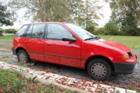
Here are the quantities I measured for my car (a 1992 Geo Metro):

M = 1000 kg (about 850kg curb weight plus 150 kg of occupants)
A = 2.3 m² (a reasonable approximation based on measurements of my car)

A plot of velocity vs time is shown below. It is based on the averages from my 6 trials. You can see that the model curve closely matches the data points.

The values of Cd and Crr for the model are:

Cd = 0.370
Crr = 0.0106

Therefore, these are the drag coefficient and coefficient of rolling resistance calculated for my car.

These values are nice to know. However, in practice, if you want to compare performance before and after making modifications to your car, you can get faster results just by measuring the time to decelerate from speed A to speed B. Pick high to medium speeds if your modifications are likely to affect drag. Pick medium to low speeds if your modifications are likely to affect rolling resistance. Don’t forget to take multiple measurements in each direction and average the results.

For more experiments you can do on your car see my website IWillTry.org .

Update 2009-01-02

I’ve learned a lot since originally posting this 16 months ago. I’ve played with measuring Cd and Crr under different conditions on a number of vehicles and other experimenters have picked apart and tweaked my spreadsheet for their own uses.

My experience is that there IS a mistake in one of the underlying assumptions of the model: namely that the force of rolling resistance is constant independent of V. Vehicles are designed with negative lift (so they get pushed into the road more at higher speeds, improving handling) so the force of rolling resistance also has a component that varies with V like the drag force. The force of rolling resistance also includes a small component of viscous force (drivetrain) which varies with V.

The model assumes that the drag force is related only to V² and that the force of rolling and drivetrain resistance is constant. In reality the force of rolling and drivetrain resistance is also related to V2 and V. So a better model of the force on a moving vehicle is:

F = iV² + jV + k where i, j, and k are constants.

A curve based on that model more closely matches actual coast down data indicating it is a more accurate model. But after solving for i, j and k, there is no way to extract meaningful values of Cd and Crr since by definition, they assume i is related only to drag, and j is 0, neither of which is entirely true. To think of it another way, Cd and Crr values define a model which is only an approximation of the real world. A physical object doesn’t really have a drag coefficient. Only the model of the physical object does.

As mentioned above, if you want to compare performance of a vehicle before and after making mods, the difference in coast down time itself is more meaningful than the change in Cd or Crr extracted from coast down data.