IWillTry.org

On one of my previous posts, Build a simple solar water heater, I recently received the comment below from a reader named John Hearty who built his own solar water heater following a similar design. I emailed John requesting some photos, and he was kind enough to oblige. Here are the pictures he sent me. Click on the images for higher resolution versions.

John says:

I have read your blog and another one you commented on about using Coroplast for thermal collector panels with great interest. I think Coroplast is an excellent material for a collector mainly because of it’s higher temperature tolerance. My wife tested baking a sample at 250 degrees F and it came out feeling just about as rigid as normal. We also filled it with water and put it in the freezer and it did not deform from the ice.

I am however concerned about freezing problems, more due to glued joints at the ABS pipe at the top and bottom of an assembled panel bursting. I plan to have a large holding tank of water used directly with the panels without a heat exchanger to the holding tank so I’m not too interested in using a bunch of anti-freeze. I am planning to build a drainback system using these panels, and just painting them black.

I also saw that polypropylene does not tolerate UV light well and will become brittle and break after long exposure. Coroplast can however be made special order with a UV absorber mixed in with the polypropylene. I am getting some regular Coroplast from a local sign shop that does not have the UV protection, so I’m looking into paints that absorb the UV. If the prototype works well I’ll look into getting UV protected Coroplast for additional panels.

And a couple weeks later:

My wife and I finally got one of these built and tested.  We built it as a drainback system and used plain water dyed black using pond dye.  We did not paint the panel.  We got frosted tempered glass panes from Craigslist to build this and the next ones.  We used an old hot water circulator pump also from Craigslist.

We did a 4 hour test on a clear day, readjusting the panel angle a few times during the test.  The full spreadsheet is available but I was not sure if it could be posted here.  It is a 1.814 square meter panel with 37.85 liters (10 gal) of water in the system.  We used a 55 gallon plastic drum for the tank.  The tank and hoses were not insulated.

Starting temp was 53.8 F. At the 1 hour mark the temp was 92.7 F, average power was 952 watts, 52% efficient. At 2 hours, 117 F, 768 watts, 42%. At 3 hours, 127 F, 593 watts, 33%. At 4 hours, 130 F, 464 watts, 26%.  We also did a stagnation test with no water in it, and it got up to 152 degrees F on a 45 degree day.  We are looking forward to mounting it permanently and testing reliability/longevity.  One thing we still need to do is get UV clear paint to help protect the panels from UV breakdown, and see if that affects the efficiency much.

Full panel and storage tank

Panel draining back into storage tank

Panel and storage tank showing water pump

Thanks John for sharing your results.

This is Chapter 2 in a series of posts on Hypermiling. In Chapter 1 I introduced the concept of energy flow analysis as a systematic way of investigating driving techniques and vehicle modifications for improved mileage. I am  considering a vehicle as a closed system with energy input in the form of fuel and several energy outputs as shown in the following energy flow diagram:

In this post I will look at the only energy input: fuel.

Work, Energy, and Power

Before looking at fuel, it’s worth defining a few terms that I will be using throughout this series of posts. “Work”, “energy”, and “power” are terms used frequently and sometimes interchangeably by the general populace, but in an engineering context, they have specific meanings that must be understood. For a greater understanding than I provide here, follow the links to Wikipedia articles.

Work is a force applied over some distance. The amount of work is equal to the force multiplied by the distance. If force is measured in Newtons (N) and distance is measured in metres, then multiplying force by distance will give work in Joules (J). The Joule is a measure of energy. Work is a specific kind of energy. It can be thought of as energy used to move something.

Energy is a measure of the capacity to do work. It is also measured in Joules. Energy can take many forms (e.g., chemical, light, heat, work). Energy can be converted from one form to another through various means. In an engine, for example, the chemical energy of a fuel is converted to heat through the process of combustion and the heat is used to expand a gas against a piston, converting some of the heat to work.

Power is a “rate” of energy flow. Power is measured in Watts (W). It can be expressed as energy per unit time. 1 Watt is equivalent to 1 Joule per second. Since work is a form of energy equal to force times distance, and power is equal to energy divided by time, it follows that power is equal to force times distance divided by time. In other words, power is equal to force times velocity.

Just as power can be expressed as energy per unit time (e.g., 1W = 1J/s), energy may be expressed as power multiplied by time (e.g., 1Ws = 1J, 1Wh = 3600J or 3.6kJ, 1kWh = 3.6MJ) . You may be more familiar with energy expressed in kWh as this is a common unit of measurement used on utility bills.

I cannot emphasize enough how important it is to understand these terms and the formulas relating them. Without such an understanding, hypermiling is all just trial and error.

Energy Density of Fuels

A certain volume of fuel contains a certain amount of chemical energy that can be released by combustion. Energy density is a measure of the chemical energy per unit volume or per unit mass of fuel. Energy is specified in kWh (recall 1kWh = 3.6MJ), volume is specified in litres, and mass is specified in kg. Thus energy density of fuels is commonly specified in kWh/litre or kWh/kg.

The table below shows energy densities for some fuels you may be familiar with:

I drive a gasoline vehicle, so for every litre of fuel consumed, 9kWh of energy is input to the vehicle and the law of conservation of energy requires that all energy losses in the vehicle energy flow chart above must total 9kWh. Hopefully it’s clear that the way those 9kWh of energy are divided between the various energy losses will have a significant effect on vehicle mileage. Of specific interest is the fraction of energy “spent” on overcoming rolling resistance and drag since those are the only “necessary losses” to move the vehicle.

Aside: Whenever I encounter energy specifications like this, I like to do a quick cost comparison. For example, I know from my utility bills that I pay about $0.07 per kWh for electricity. I pay about $1.00 per litre for gasoline. Since gasoline contains 9kWh per litre, I effectively pay $1.00/9 = $0.11 per kWh for gasoline. This is one among many of the reasons why I don’t burn gasoline to heat my home and why I’m considering building an electric vehicle.

Although it’s conceivable that the energy density of a fuel may be manipulated by additives, this is generally not attempted by hypermilers and would be a poor place to start for the beginner. Also note that energy density is not related to octane level.

Unfortunately it appears that our first stop on the energy flow diagram hasn’t yielded any techniques or modifications a driver can use to improve their mileage. However, the important thing to take away from this post is that the energy density of a fuel is fixed and that for gasoline specifically, it is 9kWh/litre or 12.8kWh/kg. I’ll be coming back to those numbers again in later posts to convert calculated energy losses back to litres of fuel consumed, which is what hypermilers are really interested in.

Stay tuned for Chapter 3 – Engine Losses which I promise will be more exciting since there ARE a lot of driving techniques and vehicle modifications you can use to improve engine efficiency.

This is the first in what I hope will be a series of posts on hypermiling. Expect MUCH more than the typical “Drive slow, accelerate gently, avoid braking… etc., etc., etc.” that you may have heard before (and that are often incorrect). I’m going to get technical. Consider this the introductory chapter, in which I’ll offer an explanation and general outline for what will follow.

Hyper-what?

Hypermilers are drivers who attempt (often obsessively) to extract every possible mile (or kilometre… up here in Canada) from a tank of gas, whether through driving techniques or vehicle modifications or both. I first started experimenting with hypermiling in 2007, having gleaned some information from websites and forums such as http://www.gassavers.org, http://cleanmpg.com, and http://www.ecomodder.com. I have a strong background in engineering and science (a B.A.Sc and M.Eng. from the University of British Columbia and I’ve been working in the field of Electrical and Mechanical Engineering for 12 years). Though the information on the above sites was a useful starting point, I found that much of it is was obvious and much of the rest of it was misguided. Some techniques are presented that produce good results, and there are certainly many members achieving excellent mileage, but the explanations given for the phenomena at work sometimes make my eyes roll. In a forum format it is difficult for an average reader to distinguish voices worth listening to from those that aren’t. My experience has been that there is a general lack of understanding of the science behind hypermiling and there is no single source where the science is explained in detail. That is something that I hope to correct through this series of posts.

Why do it?

First, let’s state the obvious. If you want to consume less fuel, the surest way to do it is to drive less. However, even walking and biking result in fuel consumption. I’ve heard it said that a meat-eating cyclist is responsible for more fossil fuel consumption per mile traveled than a vegetarian SUV driver. While I’m not certain of the validity of that statement, it does illustrate a point. A person’s effective fossil fuel consumption goes well beyond what they burn directly. In any case, the intent of this guide is not to discuss the merits of driving or not driving. I will leave it to the reader to determine that for themselves.

If you do drive I will assume you may be interested in reducing your fuel consumption. Perhaps you wish to save money. Perhaps you wish to save the environment. Perhaps you wish to reduce your dependence on foreign oil. Perhaps you are just looking for a worthy obsession. One of the best explanations for hypermiling I’ve seen comes from MetroMPG (an active member of several online forums – see his website at http://www.metrompg.com). He says:

No, it’s not just for the money.

I calculate fuel consumption on each tank of gas because it’s a challenge. It’s a high performance activity; a technical skill; a game, like GT4 and sail boat racing.

In my university days, I took a number of car racing courses. All of which boiled down to: “how to apply a few rules of physics to your driving technique in order to squeeze the maximum possible speed from a given radius, without skidding off into the weeds.” The feedback was hearing the tires sing just the right song through the curves, and out-pacing other drivers in identical cars.

Economy driving is just a different kind of performance driving: “how to apply a few rules of physics to your driving technique in order to squeeze the maximum possible distance from a given amount of fuel.” The feedback is the numbers at each fill-up, and (hopefully) beating the ratings. Plus the satisfaction of knowing it’s much easier on the machinery, the environment, and the wallet (if you don’t go overboard with efficiency mods).

It doesn’t have the instant gratification of screaming through the curves… but it’s not going to cost me my license either. Driving at the limit of grip is something safely done on the track, but driving efficiently is a game you can play anywhere, all the time.

Does it really work?

Given the number of fuel saving scams out there, I wouldn’t be surprised if you’re skeptical. I was skeptical when I started too. I had heard it said by many that the most significant gains could be had simply by changing one’s driving style. I thought I was an “economic” driver and I was skeptical that I could achieve significant improvements just by changing the way I drove. After a little research, calculation and experimentation I discovered just how wrong I was. In hindsight it seems obvious. The way we are taught to drive – the way auto manufacturers intend their vehicles to be driven – simply isn’t an efficient way of converting fuel to kilometres. In the first year after I started hypermiling, I improved my mileage from 40 MPG to 65 MPG without any vehicle modifications other than the addition of a vacuum gauge (the proper use of which I will describe in Chapter 3). In the remainder of this series I hope to describe how you too can squeeze the maximum possible distance from a given amount of fuel, under real world driving conditions, without annoying nearby drivers (well… not too much anyway) and without spending more on vehicle modifications than you’re likely to save on fuel.

It’s all about energy

Hypermiling is all about conserving energy. Thus it can best be understood through a systematic exploration of the energy flows in a vehicle. The first law of thermodynamics, often referred to as the law of conservation of energy, states that for a closed system whose internal energy remains constant, the total energy input must exactly equal the total energy output. Energy in = Energy out. Considering a vehicle as a closed system, energy is input in form of fuel. Energy flows through the system from engine to gearbox to drivetrain to wheels, etc. At each step along this flow, some energy is output from the system in the form of heat. Thus there are many paths through which energy is output from the system. The energy flow can be represented graphically as I have done in the diagram below.

The first law of thermodynamics requires that for a given distance traveled, the combined total of all energy outputs in the above diagram must exactly equal the energy input in the form of fuel.

Aside: The astute observer may note that the underlying assumption that the internal energy of the system is constant isn’t entirely true. The speed of the vehicle, the level of charge of the battery and the altitude all affect the internal energy of the system. However, these effects can be ignored as long as the vehicle is in the same state (same speed, altitude and level of charge of the battery) whenever the energy inputs and outputs are measured. Note that the amount of fuel in the tank does NOT affect the internal energy of the system since I am considering the gas tank as being OUTSIDE the system. Instead, I consider fuel as entering the system when it passes through the fuel injector. This allows more precise comparison of input to output energy and does not require that we consider the fuel in the tank as an internal energy of the system.

Note that to move a vehicle, the only losses which MUST be overcome are rolling resistance and air resistance (drag). If you were to push a vehicle by hand instead of driving it, you would be supplying the energy input. Rolling resistance and drag would be the only energy losses. Rolling resistance and drag are losses imposed by the environment from outside the system. All other losses are just an indirect result of the methods employed within the system in an attempt to overcome rolling resistance and drag.

A certain amount of fuel consumption can be attributed to each energy loss. It is a useful analogy to think of each energy loss path as a virtual hole in a your gas tank that fluctuates in size in response to your actions (vehicle speed, engine RPM, engine load, braking habits, etc). Every drop of fuel you put in your tank eventually exits the system through one of these “holes”. Hypermiling, at its heart, is the art and science of plugging the holes (at least partially) through driving techniques and vehicle modifications. The remainder of this series will be a systematic exploration of the energy inputs and outputs shown above. I will attempt to follow the outline below (I’ll change these to links as I post new information):

Chapter 1 – Introduction and outline
Chapter 2 – Fuel
Chapter 3 – Engine Losses
Chapter 4 – Drivetrain Losses
Chapter 5 – Braking Losses
Chapter 6 – Rolling Resistance
Chapter 7 – Air Resistance (Drag)
Chapter 8 – Alternator and Electrical Losses
Chapter 9 – Miscellaneous Additional Losses
Chapter 10 – Summary

Hopefully I will be able to post a chapter every couple weeks. In each chapter I’ll discuss:
1. The science that describes the phenomenon including the equations governing the energy flow.
2. How to measure the energy losses on your own vehicle to determine parameter values for the equations.
3. Driving techniques and vehicle modifications to reduce the energy losses.
4. The degree of reduction achievable for the particular energy loss, and the effect on overall fuel consumption.
5. Results from some of my own experiments.

If you have comments related to topics that I haven’t covered yet, please save them until the related topic is posted. Consider subscribing to my RSS feed and/or email notifications via the link on the main page if you want to be notified as each chapter is posted.

Stay tuned.

A moisture problem

We (my wife and I that is) keep the temperature in our home relatively low in winter. As I’m writing this, it’s a balmy 16 degrees C in my living room. My lovely wife is wearing a toque and she’s about to put on another sweater because she’s feeling “a bit of a chill”, but she’s a trooper and wouldn’t have it any other way. That’s how she was raised. In Richmond, BC, where we live, winters are… well… wet. It’s pretty much a case of 100% relative humidity outside 24/7 and the water table is at ground level… well… truthfully sometimes it’s a few feet above ground level, but that’s why we have the pumps.

Combine 100% relative humidity outside with low temperatures inside and as you might expect, we occasionally have issues with condensation, especially on windows. “Experts” generally don’t recommend keeping interior temperatures below about 17 degrees C for exactly this reason. I don’t care much for expert opinions (experience has convinced me that I’m more expert than most of them), but I also don’t care much for condensation.

A solution with a bonus: free energy

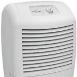
The solution (without simply raising the temperature of our home),  is a dehumidifier. While I purchased it for its intended purpose (to reduce humidity levels) I now realize that it also makes a very effective heater. Ah… but doesn’t it cost money and energy to operate a dehumidifier? Well… actually… NO! At least not in the winter, when we’re heating our home with electricity anyway. In fact, a dehumidifier is MORE efficient than an ordinary electric heater, which is already 100% efficient. Yes, a dehumidifier is more than 100% efficient at heating your home. That is to say the amount of heat a dehumidifier will release into your home is greater than the amount of electrical energy it will consume. The reason is simple: a dehumidifier removes energy from water vapor in the air in order to condense it to a liquid. This energy is released into your home.

It’s all about enthalpy

There is a property of any substance known as the enthalpy of vaporization. “Enthalpy” really just means energy. The enthalpy of vaporization of a substance is a measure of how much energy it takes to convert a given mass of the substance from a liquid to a gas. It also indicates how much energy is released when a given mass of the substance is condensed from a gas to a liquid. The enthalpy of vaporization of water is 2257 kJ/kg.

What is the efficiency?

How efficient is a dehumidifier at heating your home? Let’s figure it out together. I mean that literally. As I write this, I haven’t actually figured it out yet myself. I’m flying by the seat of my pants here, people; I’m a scientist gone rogue. But luckily I’m also a scientist who recently acquired a portable dehumidifier. I plugged it into a Kill-A-Watt meter several hours ago to measure exactly how much electrical energy (indicated in kWh by the Kill-A-Watt meter) it consumed. It’s been running for about 8 hours and it has consumed 3.87 kWh of electricity. Thus, based on the first law of thermodynamcis I know it has put at least 3.87 kWh of heat into my home.

However I have also determined with a simple digital scale that it has condensed 3.23 kg of water in that same time. How much additional energy did it release into my home as a result of that? That’s where the enthalpy of vaporization comes in. 3.23 kg multiplied by the enthalpy of vaporization of water (2257 kJ/kg) gives 7290 kJ of energy. A kWh is equivalent to 3600 kJ so 7290 kJ is equivalent to 2.025 kWh.

Thus, the total amount of heat released into my home by the dehumidifier over the last 8 hours is equivalent to the 3.87 kWh of electricity consumed, plus the 2.025 kWh of energy released by the condensation of water. The “efficiency” is equal to the energy output divided by the energy input or in this case (3.87 + 2.025)/3.87 = 1.52 or 152% efficiency. An efficiency over 100% is more appropriately referred to as a “coefficient of performance” since technically, it is impossible to achieve greater than 100% efficiency (having more than 100% efficiency in energy conversion would defy the first law of thermodynamics). So if you ever measure more than 100% efficiency, as I just did, what it really means is that you have moved energy from one place to another rather than simply converted energy from one form to another. Such is the case with a dehumidifier which removes energy from water vapor and releases it into the home in the form of heat, condensing the water to liquid in the process. But whatever the terminology you want to use, the fact remains that I can release 1.52 kWh of heat into my home for every  1 kWh of electricity my dehumidifier consumes.

What’s the payback time?

I paid about $250 CAD for my dehumidifier. It consumes about 480W of electricity (3.87 kWh in 8 h) and outputs about 730W of heat (480W*1.52) into my home. I can buy a decent electric heater that will output 730W for about $50. So the difference in price is about $200. Let’s calculate the difference in the cost to operate. A 730W electric heater consumes exactly 730W of electricity. The dehumidifier only consumes 480W of electricity to produce the same 730W of heat. The difference (730-480) is 250W. Effectively I get a free kWh (1000 Wh)of heat for every 4 hours of operation. I currently pay about $0.07 per kWh for electricty, so I save about $0.42 per day when operating the dehumidifier in place of a heater. My heating season runs from October through March, or around 180 days of the year. Therefore, I can save about 180*$0.42 = $75 per year by operating the dehumidifier in place of a heater. That will take a little over 2.5 years to pay back the difference in price of $200.

Will this work for anyone?

In a word, “No”. The human body is most comfortable at a relative humidity between 20% and 60%. I can run my dehumidifier continuously in winter and not expect to ever drop below 20% relative humidity inside my home. The same may not be true for homeowners in other locations maintaining their homes at higher temperatures than I do. Heating with a dehumidifier works for me because of the high relative humidity in Richmond, even in the winter, and because of the low temperature at which I keep the interior of my home. It could work well for anyone who lives in a similar environment and keeps their home at a low temperature. But if you live where temperatures are usually below 0 degrees C outside in winter then you likely have a much lower relatively humidity. In that case, a dehumidifier will not be able to condense nearly as much water for a given amount of input energy and its operation may bring the relative humidity below a comfortable level.

Clothes dryer vs a rack and a dehumidifier

If you’re considering hanging your wet clothing to dry inside your home, vs using your drier, then you should know that a dehumidifier will be far more efficient than a clothes dryer. In the case of a clothes dryer, electrical energy is used to vaporize the water in your clothing and the water vapor (and all the energy you’ve put into it) is expelled from your home through your drier vent. There is a net loss of energy from your home. If instead you use a dehumidifier, the heat already in your home is used to vaporize (evaporate) the water in your clothing. This energy is recaptured by the dehumidifier when the water vapor is condensed to liquid. Unlike the drier, the dehumidifier doesn’t expel any energy from your home.

Heat pump vs dehumidifier

A dehumidifier is effectively a heat pump. Rather than extracting heat from the ground or the outside air, a dehumidifier extracts heat from water vapor contained in a home’s inside air. In my home, for reasons given above, I can run my dehumidifier continuously without reducing the relative humidity in my home below a comfortable level and I’ve found the coefficient of performance (COP) is about 1.52. A typical air source heat pump has a COP of around 4 assuming an outside temperature of around 0 degrees C (a typical Richmond winter). A typical ground source heat pump has a COP of around 7 assuming a ground temperature of around 10 degrees C (a typical Richmond ground temperature). So clearly, a heat pump (either air or ground source) is much more efficient. If I had a heat pump, I would be consuming more energy than otherwise by operating my dehumidifier. That said, I feel secure in the knowledge that I can run my single dehumidifier continously and consume less energy to heat my home than if I were running an electric heater. I’ll save the installation of a heat pump for another day… perhaps.

Can you heat your whole home this way?

No. If I were to install more portable dehumidifiers to provide all the heat my home requires (to maintain a balmy 16 degrees C all winter long) I would almost certainly bring the relative humidity below comfortable levels, and the COP would drop below the measured value of 1.52 simply because there isn’t enough water vapor in the air to be condensed. So the idea of using a dehumidifier to heat one’s home is clearly not scalable. At best a dehumidifier may provide suplemental heat. I think  I might get away with using two portable dehumidifiers continuously which would each save me about $75 per year based on the calculations above. That’s about $150 per year in total. Currently, that’s about 10% of my home’s annual heating bill.

Purpose

The purpose of this experiment is to determine your vehicle’s drag coefficient Cd and coefficient of rolling resistance Crr. This is done by measuring your vehicle’s speed as a function of time while coasting in neutral (also known as a coast down test).

Why would you want to know Cd and Crr for your vehicle? Well, suppose you’re interested in modifying your vehicle for improved fuel efficiency. You might consider modifications such as air dams, wheel skirts, removing mirrors, switching to low rolling resistance tires, etc. Cd and Crr offer a quantitative method of comparing vehicle performance before and after these types of modifications to see if you made any improvement.

Equipment

You will need the following equipment:

• a vehicle (and someone with a driver’s license)
• a clock or stopwatch
• a pen and paper (and someone other than the driver to record data)
• a flashlight (driving at night avoids traffic)
• a long stretch of flat road with little traffic or wind
• Excel or another spreadsheet application. I prefer OpenOffice Calc which you can download and use for free, but its Solver function does not handle non-linear systems (yet) so you’ll have adjust input variables manually by an iterative process to minimize the error between the model curve and your data (it’s not too hard, I promise).
• The spreadsheet I created to analyze the results. You can download it here: Drag_Coefficient.xls

Background Information

First, let’s define some quantities:

Fd is the force on the vehicle due to air resistance (drag) in Newtons
Frr is the force on the vehicle due to rolling resistance in Newtons
F is the total force on the vehicle in Newtons
V is the vehicle’s velocity in m/s
a is the vehicle’s acceleration in m/s²
A is vehicle frontal area in m²
M is vehicle mass including occupants in kg
rho is the density of air which is 1.22 kg/m³ at sea level
g is the gravitational acceleration constant which is 9.81 m/s²
Cd is the vehicle’s drag coefficient we want to determine
Crr is the vehicle’s coefficient of rolling resistance we want to determine

Now for some formulas:

Fd = -Cd*A*0.5*rho*V² (formula for force due to air resistance or drag)
Frr = -Crr*M*g (formula for force due to rolling resistance)
F = Fd + Frr (total force is the sum of Fd and Frr)
F = M*a (Newton’s second law)

Note that both Fd and Frr are negative indicating that these forces act opposite to the direction of the velocity. Note also that Fd is increases as the square of velocity. This is why driving at high speeds is much less efficient than driving at low speeds. Combining these formulas with a bit of algebra gives us the acceleration due to air and wind resistance as a function of velocity:

a = -(Cd*A*0.5*rho*V²)/M – Crr*g

Note that the acceleration is negative indicating that air and wind resistance will cause the velocity to decrease.

I created my spreadsheet (see Equipment section above for download) based on these formulas to generate a model of velocity vs time that can be compared to actual data. The model values for Cd and Crr can thus be adjusted until the model matches the data. This adjustment can be done manually, by overwriting the values of Cd and Crr with new values till the model matches the data, or it can be done using a “Solver” function.

Procedure

You can determine Cd and Crr from the same set of test data by measuring velocity with respect to time as your vehicle coasts in neutral. Note that Crr will not be pure rolling resistance but will include some drive-train resistance as well.

1. Drive to a flat road with little traffic or wind.

2. Have the passenger ready with stopwatch and paper to record data.

3. Have the driver accelerate up to above 70 km/h or so, and shift into neutral.

4. Record data as follows. The driver should indicate when the speed drops to exactly 70 km/h. At this time (t=0) the passenger should start the clock. The passenger should indicate every 10 seconds after that and the driver should call out the current speed to the nearest whole km. The passenger should record this value next to each time.

Aside: If you have a digital camera capable of recording several minutes of low resolution video (as most people seem to have these days), the process is much easier and more accurate. You don’t need any equipment except the digital camera. Simply have your passenger record a video of your speedometer during the coast down tests, or find some way of mounting the camera so you can do the recording without an assistant. Using a free program such as Avidemux (http://fixounet.free.fr/avidemux/) you can play the video back on your computer frame by frame and view the speeds at desired times.

5. Repeat the test in the opposite direction.

6. Repeat the test in both directions twice more (6 trials in all, 3 in each direction). All these values will be averaged for a more accurate analysis.

7. Download the spreadsheet I created (see Equipment section above) and enter all your data following the instructions included. The spreadsheet averages data from all 6 trials to create a single data set representing velocity (V actual) as a function of time. It then generates it’s own model for velocity (V model) based on entered constants and initial guesses for Cd and Crr. Excel’s “Solver” function can be used to adjust Cd and Crr in order to minimize the error between the model and actual data. If you are using OpenOffice Calc (which I highly recommend and which you can download for free from http://www.openoffice.org ), unfortunately, the solver function currently only handles linear systems, so you will have to adjust the input values manually to minimize the error between the model and the data. Once the error is minimized and the model data matches the actual data as best it can, then Cd and Crr are correct.

Results

Here are the quantities I measured for my car (a 1992 Geo Metro):

M = 1000 kg (about 850kg curb weight plus 150 kg of occupants)
A = 2.3 m² (a reasonable approximation based on measurements of my car)

A plot of velocity vs time is shown below. It is based on the averages from my 6 trials. You can see that the model curve closely matches the data points.

The values of Cd and Crr for the model are:

Cd = 0.370
Crr = 0.0106

Therefore, these are the drag coefficient and coefficient of rolling resistance calculated for my car.

These values are nice to know. However, in practice, if you want to compare performance before and after making modifications to your car, you can get faster results just by measuring the time to decelerate from speed A to speed B. Pick high to medium speeds if your modifications are likely to affect drag. Pick medium to low speeds if your modifications are likely to affect rolling resistance. Don’t forget to take multiple measurements in each direction and average the results.

For more experiments you can do on your car see my website IWillTry.org .

Update 2009-01-02

I’ve learned a lot since originally posting this 16 months ago. I’ve played with measuring Cd and Crr under different conditions on a number of vehicles and other experimenters have picked apart and tweaked my spreadsheet for their own uses.

My experience is that there IS a mistake in one of the underlying assumptions of the model: namely that the force of rolling resistance is constant independent of V. Vehicles are designed with negative lift (so they get pushed into the road more at higher speeds, improving handling) so the force of rolling resistance also has a component that varies with V like the drag force. The force of rolling resistance also includes a small component of viscous force (drivetrain) which varies with V.

The model assumes that the drag force is related only to V² and that the force of rolling and drivetrain resistance is constant. In reality the force of rolling and drivetrain resistance is also related to V2 and V. So a better model of the force on a moving vehicle is:

F = iV² + jV + k where i, j, and k are constants.

A curve based on that model more closely matches actual coast down data indicating it is a more accurate model. But after solving for i, j and k, there is no way to extract meaningful values of Cd and Crr since by definition, they assume i is related only to drag, and j is 0, neither of which is entirely true. To think of it another way, Cd and Crr values define a model which is only an approximation of the real world. A physical object doesn’t really have a drag coefficient. Only the model of the physical object does.

As mentioned above, if you want to compare performance of a vehicle before and after making mods, the difference in coast down time itself is more meaningful than the change in Cd or Crr extracted from coast down data.